If you are a reservoir Engineer or collaborate with reservoir engineers you must have heard of Decline Curve Analysis (DCA). But what’s DCA anyway?
DCA is an empirical graphical technique which is used to forecast oil and gas production and estimate the remaining reserve. The goal of DCA is to extract useful information for asset management purposes from production rate measurements.
Empirical DCA is one of the most popular methods to forecast production and estimate EUR from previous production. While Equations derived by Arps have been the backbone of DCA for several years, in recent years new DCA methods were proposed by others to predict rate with higher certainty especially in unconventional reservoirs.
Hamza Ali, Reservoir Engineer
Popular Decline Curve Models
1. Arps
Arps’ DCA is an empirical method based on the plot of flow rate versus time to the abandonment time. There are three types of production rate decline characterized based on the way in which rate declines with time: hyperbolic, harmonic, and exponential.
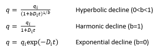
where qi is the maximum production rate (usually is equal to instantaneous rate at time 0), q is the instantaneous producing rate at time t, Di is the initial decline rate at time 0, and b is the power exponent which controls how the change of the decline rate with time. The value of b is 1 and 0 for harmonic and exponential declines, respectively. b changes in the range of 0 to 1 for hyperbolic decline. For unconventional resources sometimes b values greater than 1 is used for analyzing production data.
2. PLE
Power Law Exponential was developed by Ilk et al. in 2008 to forecast production in shale reservoirs.
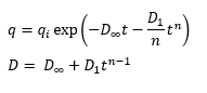
where D∞ is decline rate at large times, D1 is initial decline rate, and n is hyperbolic exponent (0 <= n <= 0.5).
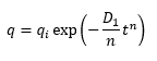
3. SEPD
SEPD was proposed by Valko in 2008 and is very similar to PLE. The only difference between SEPD and PLE is in the late time of production because for SEPD method the D∞ is equal to zero.
4. Duong
Another method to forecast production in shale reservoirs was proposed by Duong in 2011.
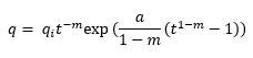
where a and m are the slope and intercept of the rate over cumulative production plotted versus time, respectively.
5. LGM
Logistic Growth Model (Clark et al. 2011) is based on the concept that decline rate grows only to a certain size in time. In DCA analysis the maximum recoverable reserve is EUR. The sum of the remaining reserve and cumulative production for a fixed economic rate limit must not exceed EUR. The maximum growth size (in this case EUR) is called carrying capacity, K.
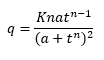
where K is carrying capacity, n is a parameter than controls the steepness of the decline curve, and a is the decline exponent.
Above is a DCA simulation hosted on the metaKinetic platform. Using this application you can determine the cumulative production, remaining reserve, and estimated ultimate recovery (EUR) from graphical decline curve analysis using all models named above in different phases such as gas, oil, water.
Want access to this simulation and more on the metaKinetic platform? Contact us!